Fitting a piecewise-exponential model (PEM) to simulated data
In [2]:
%load_ext autoreload
%autoreload 2
%matplotlib inline
import random
random.seed(1100038344)
import survivalstan
import numpy as np
import pandas as pd
from stancache import stancache
from matplotlib import pyplot as plt
INFO:stancache.seed:Setting seed to 1245502385
The autoreload extension is already loaded. To reload it, use:
  %reload_ext autoreload
The model
This style of modeling is often called the “piecewise exponential model”, or PEM. It is the simplest case where we estimate the hazard of an event occurring in a time period as the outcome, rather than estimating the survival (ie, time to event) as the outcome.
Recall that, in the context of survival modeling, we have two models:
- A model for Survival (:math:`S`), ie the probability of surviving to time \(t\):
- A model for the instantaneous *hazard* :math:`lambda`, ie the probability of a failure event occuring in the interval [\(t\), \(t+\delta t\)], given survival to time \(t\):
By definition, these two are related to one another by the following equation:
Solving this, yields the following:
This model is called the piecewise exponential model because of this relationship between the Survival and hazard functions. It’s piecewise because we are not estimating the instantaneous hazard; we are instead breaking time periods up into pieces and estimating the hazard for each piece.
There are several variations on the PEM model implemented in
survivalstan. In this notebook, we are exploring just one of them.
A note about data formatting
When we model Survival, we typically operate on data in time-to-event
form. In this form, we have one record per Subject (ie, per
patient). Each record contains [event_status, time_to_event] as the
outcome. This data format is sometimes called per-subject.
When we model the hazard by comparison, we typically operate on data
that are transformed to include one record per Subject per
time_period. This is called per-timepoint or long form.
All other things being equal, a model for Survival will typically estimate more efficiently (faster & smaller memory footprint) than one for hazard simply because the data are larger in the per-timepoint form than the per-subject form. The benefit of the hazard models is increased flexibility in terms of specifying the baseline hazard, time-varying effects, and introducing time-varying covariates.
In this example, we are demonstrating use of the standard PEM survival
model, which uses data in long form. The stan code expects to
recieve data in this structure.
Stan code for the model
This model is provided in survivalstan.models.pem_survival_model.
Let’s take a look at the stan code.
In [3]:
print(survivalstan.models.pem_survival_model)
/*  Variable naming:
 // dimensions
 N          = total number of observations (length of data)
 S          = number of sample ids
 T          = max timepoint (number of timepoint ids)
 M          = number of covariates

 // main data matrix (per observed timepoint*record)
 s          = sample id for each obs
 t          = timepoint id for each obs
 event      = integer indicating if there was an event at time t for sample s
 x          = matrix of real-valued covariates at time t for sample n [N, X]

 // timepoint-specific data (per timepoint, ordered by timepoint id)
 t_obs      = observed time since origin for each timepoint id (end of period)
 t_dur      = duration of each timepoint period (first diff of t_obs)

*/
// Jacqueline Buros Novik <jackinovik@gmail.com>

data {
  // dimensions
  int<lower=1> N;
  int<lower=1> S;
  int<lower=1> T;
  int<lower=0> M;

  // data matrix
  int<lower=1, upper=N> s[N];     // sample id
  int<lower=1, upper=T> t[N];     // timepoint id
  int<lower=0, upper=1> event[N]; // 1: event, 0:censor
  matrix[N, M] x;                 // explanatory vars

  // timepoint data
  vector<lower=0>[T] t_obs;
  vector<lower=0>[T] t_dur;
}
transformed data {
  vector[T] log_t_dur;  // log-duration for each timepoint
  int n_trans[S, T];

  log_t_dur = log(t_obs);

  // n_trans used to map each sample*timepoint to n (used in gen quantities)
  // map each patient/timepoint combination to n values
  for (n in 1:N) {
      n_trans[s[n], t[n]] = n;
  }

  // fill in missing values with n for max t for that patient
  // ie assume "last observed" state applies forward (may be problematic for TVC)
  // this allows us to predict failure times >= observed survival times
  for (samp in 1:S) {
      int last_value;
      last_value = 0;
      for (tp in 1:T) {
          // manual says ints are initialized to neg values
          // so <=0 is a shorthand for "unassigned"
          if (n_trans[samp, tp] <= 0 && last_value != 0) {
              n_trans[samp, tp] = last_value;
          } else {
              last_value = n_trans[samp, tp];
          }
      }
  }
}
parameters {
  vector[T] log_baseline_raw; // unstructured baseline hazard for each timepoint t
  vector[M] beta;         // beta for each covariate
  real<lower=0> baseline_sigma;
  real log_baseline_mu;
}
transformed parameters {
  vector[N] log_hazard;
  vector[T] log_baseline;     // unstructured baseline hazard for each timepoint t

  log_baseline = log_baseline_mu + log_baseline_raw + log_t_dur;

  for (n in 1:N) {
    log_hazard[n] = log_baseline[t[n]] + x[n,]*beta;
  }
}
model {
  beta ~ cauchy(0, 2);
  event ~ poisson_log(log_hazard);
  log_baseline_mu ~ normal(0, 1);
  baseline_sigma ~ normal(0, 1);
  log_baseline_raw ~ normal(0, baseline_sigma);
}
generated quantities {
  real log_lik[N];
  vector[T] baseline;
  real y_hat_time[S];      // predicted failure time for each sample
  int y_hat_event[S];      // predicted event (0:censor, 1:event)

  // compute raw baseline hazard, for summary/plotting
  baseline = exp(log_baseline_mu + log_baseline_raw);

  // prepare log_lik for loo-psis
  for (n in 1:N) {
      log_lik[n] = poisson_log_log(event[n], log_hazard[n]);
  }

  // posterior predicted values
  for (samp in 1:S) {
      int sample_alive;
      sample_alive = 1;
      for (tp in 1:T) {
        if (sample_alive == 1) {
              int n;
              int pred_y;
              real log_haz;

              // determine predicted value of this sample's hazard
              n = n_trans[samp, tp];
              log_haz = log_baseline[tp] + x[n,] * beta;

              // now, make posterior prediction of an event at this tp
              if (log_haz < log(pow(2, 30)))
                  pred_y = poisson_log_rng(log_haz);
              else
                  pred_y = 9;

              // summarize survival time (observed) for this pt
              if (pred_y >= 1) {
                  // mark this patient as ineligible for future tps
                  // note: deliberately treat 9s as events
                  sample_alive = 0;
                  y_hat_time[samp] = t_obs[tp];
                  y_hat_event[samp] = 1;
              }

          }
      } // end per-timepoint loop

      // if patient still alive at max
      if (sample_alive == 1) {
          y_hat_time[samp] = t_obs[T];
          y_hat_event[samp] = 0;
      }
  } // end per-sample loop
}
This may seem pretty intimidating, but once you get used to the Stan language you may find it’s pretty powerful.
One of the goals of `survivalstan <>`__ is to allow you to edit the stan code directly, if you choose to do so. Or to reference Stan code for models others have written. This expands the range of what `survivalstan <>`__ can do.
Simulate survival data
In order to demonstrate the use of this model, we will first simulate
some survival data using survivalstan.sim.sim_data_exp_correlated.
As the name implies, this function simulates data assuming a constant
hazard throughout the follow-up time period, which is consistent with
the Exponential survival function.
This function includes two simulated covariates by default (age and
sex). We also simulate a situation where hazard is a function of the
simulated value for sex.
We also center the age variable since this will make it easier to
interpret estimates of the baseline hazard.
In [4]:
d = stancache.cached(
    survivalstan.sim.sim_data_exp_correlated,
    N=100,
    censor_time=20,
    rate_form='1 + sex',
    rate_coefs=[-3, 0.5],
)
d['age_centered'] = d['age'] - d['age'].mean()
INFO:stancache.stancache:sim_data_exp_correlated: cache_filename set to sim_data_exp_correlated.cached.N_100.censor_time_20.rate_coefs_21453428780.rate_form_1 + sex.pkl
INFO:stancache.stancache:sim_data_exp_correlated: Starting execution
INFO:stancache.stancache:sim_data_exp_correlated: Execution completed (0:00:00.024619 elapsed)
INFO:stancache.stancache:sim_data_exp_correlated: Saving results to cache
*Aside: In order to make this a more reproducible example, this code is
using a file-caching function stancache.cached to wrap a function
call to survivalstan.sim.sim_data_exp_correlated. *
Explore simulated data
Here is what these data look like - this is per-subject or
time-to-event form:
In [5]:
d.head()
Out[5]:
| age | sex | rate | true_t | t | event | index | age_centered | |
|---|---|---|---|---|---|---|---|---|
| 0 | 39 | male | 0.082085 | 14.798745 | 14.798745 | True | 0 | -16.33 |
| 1 | 47 | female | 0.049787 | 2.613670 | 2.613670 | True | 1 | -8.33 |
| 2 | 53 | female | 0.049787 | 81.586870 | 20.000000 | False | 2 | -2.33 |
| 3 | 54 | male | 0.082085 | 17.647537 | 17.647537 | True | 3 | -1.33 |
| 4 | 49 | male | 0.082085 | 6.346437 | 6.346437 | True | 4 | -6.33 |
It’s not that obvious from the field names, but in this example “subjects” are indexed by the field ``index``.
We can plot these data using lifelines, or the rudimentary plotting
functions provided by survivalstan.
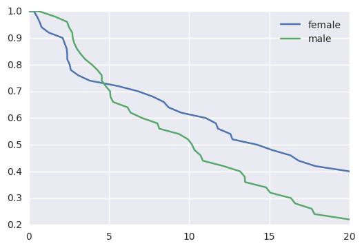
In [6]:
survivalstan.utils.plot_observed_survival(df=d[d['sex']=='female'], event_col='event', time_col='t', label='female')
survivalstan.utils.plot_observed_survival(df=d[d['sex']=='male'], event_col='event', time_col='t', label='male')
plt.legend()
Out[6]:
<matplotlib.legend.Legend at 0x7f39e153b950>
Transform to long or per-timepoint form
Finally, since this is a PEM model, we transform our data to long or
per-timepoint form.
In [7]:
dlong = stancache.cached(
    survivalstan.prep_data_long_surv,
    df=d, event_col='event', time_col='t'
)
INFO:stancache.stancache:prep_data_long_surv: cache_filename set to prep_data_long_surv.cached.df_17750466280.event_col_event.time_col_t.pkl
INFO:stancache.stancache:prep_data_long_surv: Starting execution
INFO:stancache.stancache:prep_data_long_surv: Execution completed (0:00:00.388285 elapsed)
INFO:stancache.stancache:prep_data_long_surv: Saving results to cache
We now have one record per timepoint (distinct values of end_time)
per subject (index, in the original data frame).
In [8]:
dlong.query('index == 1').sort_values('end_time').tail()
Out[8]:
| age | sex | rate | true_t | t | event | index | age_centered | end_time | end_failure | |
|---|---|---|---|---|---|---|---|---|---|---|
| 133 | 47 | female | 0.049787 | 2.61367 | 2.61367 | True | 1 | -8.33 | 2.394245 | False |
| 80 | 47 | female | 0.049787 | 2.61367 | 2.61367 | True | 1 | -8.33 | 2.395736 | False |
| 83 | 47 | female | 0.049787 | 2.61367 | 2.61367 | True | 1 | -8.33 | 2.502706 | False |
| 125 | 47 | female | 0.049787 | 2.61367 | 2.61367 | True | 1 | -8.33 | 2.549188 | False |
| 71 | 47 | female | 0.049787 | 2.61367 | 2.61367 | True | 1 | -8.33 | 2.613670 | True |
Fit stan model
Now, we are ready to fit our model using
survivalstan.fit_stan_survival_model.
We pass a few parameters to the fit function, many of which are required. See ?survivalstan.fit_stan_survival_model for details.
Similar to what we did above, we are asking survivalstan to cache
this model fit object. See
stancache for more details on
how this works. Also, if you didn’t want to use the cache, you could
omit the parameter FIT_FUN and survivalstan would use the
standard pystan functionality.
In [10]:
testfit = survivalstan.fit_stan_survival_model(
    model_cohort = 'test model',
    model_code = survivalstan.models.pem_survival_model,
    df = dlong,
    sample_col = 'index',
    timepoint_end_col = 'end_time',
    event_col = 'end_failure',
    formula = '~ age_centered + sex',
    iter = 5000,
    chains = 4,
    seed = 9001,
    FIT_FUN = stancache.cached_stan_fit,
    )
INFO:stancache.stancache:Step 1: Get compiled model code, possibly from cache
INFO:stancache.stancache:StanModel: cache_filename set to anon_model.cython_0_25_2.model_code_5118842489520038317.pystan_2_14_0_0.stanmodel.pkl
INFO:stancache.stancache:StanModel: Loading result from cache
INFO:stancache.stancache:Step 2: Get posterior draws from model, possibly from cache
INFO:stancache.stancache:sampling: cache_filename set to anon_model.cython_0_25_2.model_code_5118842489520038317.pystan_2_14_0_0.stanfit.chains_4.data_14507016511.iter_5000.seed_9001.pkl
INFO:stancache.stancache:sampling: Loading result from cache
Superficial review of convergence
We will note here some top-level summaries of posterior draws – this is a minimal example so it’s unlikely that this model converged very well.
In practice, you would want to do a lot more investigation of convergence issues, etc. For now the goal is to demonstrate the functionalities available here.
We can summarize posterior estimates for a single parameter, (e.g. the
built-in Stan parameter lp__):
In [11]:
survivalstan.utils.print_stan_summary([testfit], pars='lp__')
            mean   se_mean         sd       2.5%        50%       97.5%      Rhat
lp__ -258.914979  6.067607  49.665504 -335.83595 -267.33087 -154.100868  1.085588
Or, for sets of parameters with the same name:
In [12]:
survivalstan.utils.print_stan_summary([testfit], pars='log_baseline_raw')
                          mean   se_mean        sd      2.5%       50%     97.5%      Rhat
log_baseline_raw[0]   0.019647  0.001436  0.143627 -0.265423  0.008856  0.351903  1.000186
log_baseline_raw[1]   0.017001  0.001451  0.145123 -0.276477  0.006995  0.348198  1.000221
log_baseline_raw[2]   0.017916  0.001475  0.147465 -0.283370  0.007572  0.357371  1.000288
log_baseline_raw[3]   0.017542  0.001455  0.145524 -0.276583  0.008317  0.351408  1.000975
log_baseline_raw[4]   0.017227  0.001463  0.146328 -0.278237  0.006810  0.353518  1.000206
log_baseline_raw[5]   0.014864  0.001482  0.148171 -0.289185  0.006228  0.359035  1.000175
log_baseline_raw[6]   0.012331  0.001413  0.141270 -0.275576  0.005273  0.327449  1.000171
log_baseline_raw[7]   0.007920  0.001509  0.150910 -0.304167  0.003191  0.339291  1.000073
log_baseline_raw[8]   0.008752  0.001404  0.140400 -0.274269  0.003630  0.316078  1.000433
log_baseline_raw[9]   0.008926  0.001436  0.143608 -0.286753  0.003888  0.319980  0.999990
log_baseline_raw[10]  0.009011  0.001439  0.143859 -0.289257  0.004465  0.322414  0.999994
log_baseline_raw[11]  0.004890  0.001452  0.145208 -0.306954  0.003050  0.331526  1.000125
log_baseline_raw[12]  0.008431  0.001442  0.144245 -0.285667  0.004344  0.330919  0.999826
log_baseline_raw[13]  0.008531  0.001461  0.146150 -0.300336  0.003858  0.336951  0.999741
log_baseline_raw[14]  0.007133  0.001426  0.142569 -0.292241  0.004296  0.317077  1.000004
log_baseline_raw[15]  0.007492  0.001421  0.142050 -0.287254  0.003846  0.323929  0.999866
log_baseline_raw[16]  0.008341  0.001447  0.144716 -0.285362  0.005005  0.323623  0.999916
log_baseline_raw[17]  0.006150  0.001398  0.139799 -0.287581  0.003530  0.313004  1.000583
log_baseline_raw[18]  0.006208  0.001414  0.141440 -0.287870  0.003043  0.310741  0.999955
log_baseline_raw[19]  0.004626  0.001407  0.140725 -0.286533  0.001647  0.318195  0.999982
log_baseline_raw[20]  0.007053  0.001424  0.142352 -0.298405  0.003217  0.332473  1.000008
log_baseline_raw[21]  0.006165  0.001448  0.144757 -0.301705  0.003087  0.324310  0.999954
log_baseline_raw[22]  0.003023  0.001443  0.144289 -0.299801  0.000831  0.330782  0.999736
log_baseline_raw[23]  0.003489  0.001455  0.145501 -0.308853  0.001102  0.323494  0.999748
log_baseline_raw[24]  0.004883  0.001422  0.142161 -0.302533  0.001940  0.319808  1.000362
log_baseline_raw[25] -0.000134  0.001419  0.141871 -0.311378 -0.000005  0.304250  0.999907
log_baseline_raw[26] -0.000183  0.001417  0.141678 -0.306077  0.000268  0.315511  0.999709
log_baseline_raw[27]  0.000082  0.001406  0.140576 -0.307312  0.000120  0.302780  0.999945
log_baseline_raw[28]  0.001481  0.001387  0.138691 -0.296750  0.001219  0.305398  0.999783
log_baseline_raw[29]  0.000518  0.001427  0.142696 -0.298523 -0.000299  0.306153  0.999623
log_baseline_raw[30] -0.000567  0.001401  0.140102 -0.310931  0.001061  0.290790  0.999853
log_baseline_raw[31]  0.002251  0.001418  0.141821 -0.308225  0.001303  0.306985  0.999873
log_baseline_raw[32] -0.000592  0.001458  0.145825 -0.312424  0.000043  0.316410  0.999696
log_baseline_raw[33] -0.004592  0.001385  0.138487 -0.304364 -0.002543  0.294671  0.999654
log_baseline_raw[34] -0.003992  0.001454  0.145389 -0.322561 -0.001881  0.302946  0.999755
log_baseline_raw[35] -0.004156  0.001409  0.140897 -0.306749 -0.001493  0.294782  0.999690
log_baseline_raw[36] -0.005276  0.001409  0.140950 -0.325573 -0.002215  0.291857  0.999829
log_baseline_raw[37] -0.007617  0.001415  0.141474 -0.321741 -0.002645  0.289491  0.999988
log_baseline_raw[38] -0.007937  0.001408  0.140822 -0.313421 -0.004623  0.286457  0.999982
log_baseline_raw[39] -0.007657  0.001364  0.136358 -0.312765 -0.002851  0.285250  1.000174
log_baseline_raw[40] -0.008427  0.001410  0.140992 -0.322515 -0.003162  0.282210  0.999950
log_baseline_raw[41] -0.006690  0.001425  0.142507 -0.319207 -0.002328  0.285721  0.999908
log_baseline_raw[42] -0.010126  0.001443  0.144295 -0.339026 -0.003639  0.292575  0.999805
log_baseline_raw[43] -0.008422  0.001427  0.142724 -0.336195 -0.002332  0.284262  1.000084
log_baseline_raw[44] -0.009589  0.001405  0.140526 -0.320643 -0.003248  0.274365  1.000060
log_baseline_raw[45] -0.010275  0.001418  0.141758 -0.330956 -0.003702  0.273868  1.000145
log_baseline_raw[46] -0.010149  0.001441  0.144062 -0.338806 -0.004575  0.289066  1.000731
log_baseline_raw[47] -0.010984  0.001418  0.141784 -0.330928 -0.004726  0.283092  0.999755
log_baseline_raw[48] -0.010872  0.001390  0.139015 -0.330739 -0.004454  0.280835  1.000222
log_baseline_raw[49] -0.009884  0.001403  0.140311 -0.324124 -0.004117  0.275271  0.999847
log_baseline_raw[50] -0.011829  0.001375  0.137513 -0.314276 -0.004940  0.264868  1.000077
log_baseline_raw[51] -0.011702  0.001458  0.145799 -0.336412 -0.005200  0.285959  0.999959
log_baseline_raw[52] -0.010392  0.001469  0.146867 -0.349373 -0.003537  0.283791  0.999980
log_baseline_raw[53] -0.010106  0.001403  0.140349 -0.312402 -0.003562  0.274880  0.999808
log_baseline_raw[54] -0.012862  0.001421  0.142080 -0.338375 -0.005334  0.273351  1.000034
log_baseline_raw[55] -0.011897  0.001398  0.139820 -0.332632 -0.004097  0.274485  0.999865
log_baseline_raw[56] -0.012945  0.001390  0.138961 -0.331729 -0.004685  0.270914  1.000496
log_baseline_raw[57] -0.010691  0.001411  0.141106 -0.330575 -0.005446  0.290778  0.999797
log_baseline_raw[58] -0.012159  0.001410  0.140981 -0.339378 -0.005554  0.280880  0.999786
log_baseline_raw[59] -0.012971  0.001433  0.143279 -0.334722 -0.005576  0.280169  1.000235
log_baseline_raw[60] -0.010581  0.001430  0.143014 -0.328594 -0.004387  0.279914  0.999954
log_baseline_raw[61] -0.008223  0.001426  0.142638 -0.326803 -0.003350  0.292468  0.999918
log_baseline_raw[62] -0.012020  0.001437  0.143716 -0.334068 -0.005828  0.282619  1.000157
log_baseline_raw[63] -0.009945  0.001425  0.142458 -0.325602 -0.004666  0.285909  0.999998
log_baseline_raw[64] -0.011442  0.001499  0.149850 -0.349216 -0.005765  0.309402  1.000616
log_baseline_raw[65] -0.009525  0.001438  0.143808 -0.326331 -0.004767  0.296830  1.000247
log_baseline_raw[66] -0.011176  0.001369  0.136854 -0.322828 -0.004931  0.266086  0.999885
log_baseline_raw[67] -0.009417  0.001412  0.141209 -0.327826 -0.004775  0.283079  1.000007
log_baseline_raw[68] -0.007313  0.001392  0.139212 -0.315294 -0.003673  0.284527  1.000071
log_baseline_raw[69] -0.031890  0.001490  0.149014 -0.392716 -0.014664  0.257069  1.001029
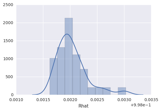
It’s also not uncommon to graphically summarize the Rhat values, to
get a sense of similarity among the chains for particular parameters.
In [13]:
survivalstan.utils.plot_stan_summary([testfit], pars='log_baseline_raw')
Plot posterior estimates of parameters
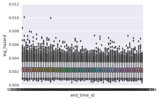
We can use plot_coefs to summarize posterior estimates of
parameters.
In this basic pem_survival_model, we estimate a parameter for
baseline hazard for each observed timepoint which is then adjusted for
the duration of the timepoint. For consistency, the baseline values are
normalized to the unit time given in the input data. This allows us to
compare hazard estimates across timepoints without having to know the
duration of a timepoint. (in general, the duration-adjusted hazard
paramters are suffixed with ``_raw`` whereas those which are
unit-normalized do not have a suffix).
In this model, the baseline hazard is parameterized by two components –
there is an overall mean across all timepoints (log_baseline_mu) and
some variance per timepoint (log_baseline_tp). The degree of
variance is estimated from the data as log_baseline_sigma. All
components have weak default priors. See the stan code above for
details.
In this case, the model estimates a minimal degree of variance across timepoints, which is good given that the simulated data assumed a constant hazard over time.
In [14]:
survivalstan.utils.plot_coefs([testfit], element='baseline')
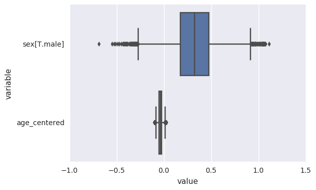
We can also summarize the posterior estimates for our beta
coefficients. This is actually the default behavior of plot_coefs.
Here we hope to see the posterior estimates of beta coefficients include
the value we used for our simulation (0.5).
In [15]:
survivalstan.utils.plot_coefs([testfit])
Posterior predictive checking
Finally, survivalstan provides some utilities for posterior
predictive checking.
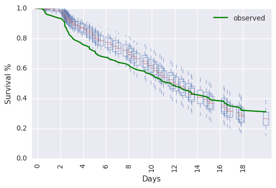
The goal of posterior-predictive checking is to compare the uncertainty of model predictions to observed values.
We are not doing true out-of-sample predictions, but we are able to sanity-check our model’s calibration. We expect approximately 5% of observed values to fall outside of their corresponding 95% posterior-predicted intervals.
By default, survivalstan‘s plot_pp_survival method will plot
whiskers at the 2.5th and 97.5th percentile values, corresponding to 95%
predicted intervals.
In [ ]:
survivalstan.utils.plot_pp_survival([testfit], fill=False)
survivalstan.utils.plot_observed_survival(df=d, event_col='event', time_col='t', color='green', label='observed')
plt.legend()
<matplotlib.legend.Legend at 0x7f3966f1d510>
We can also summarize and plot survival by our covariates of interest,
provided they are included in the original dataframe provided to
fit_stan_survival_model.
In [ ]:
survivalstan.utils.plot_pp_survival([testfit], by='sex')
This plot can also be customized by a variety of aesthetic elements
In [ ]:
survivalstan.utils.plot_pp_survival([testfit], by='sex', pal=['red', 'blue'])
Building up the plot semi-manually, for more customization
We can also access the utility methods within survivalstan.utils to
more or less produce the same plot. This sequence is intended to both
illustrate how the above-described plot was constructed, and expose some
of the functionality in a more concrete fashion.
Probably the most useful element is being able to summarize & return posterior-predicted values to begin with:
In [ ]:
ppsurv = survivalstan.utils.prep_pp_survival_data([testfit], by='sex')
Here are what these data look like:
In [ ]:
ppsurv.head()
(Note that this itself is a summary of the posterior draws returned by
survivalstan.utils.prep_pp_data. In this case, the survival stats
are summarized by values of ['iter', 'model_cohort', by].
We can then call out to survivalstan.utils._plot_pp_survival_data to
construct the plot. In this case, we overlay the posterior predicted
intervals with observed values.
In [ ]:
subplot = plt.subplots(1, 1)
survivalstan.utils._plot_pp_survival_data(ppsurv.query('sex == "male"').copy(),
                                          subplot=subplot, color='blue', alpha=0.5)
survivalstan.utils._plot_pp_survival_data(ppsurv.query('sex == "female"').copy(),
                                          subplot=subplot, color='red', alpha=0.5)
survivalstan.utils.plot_observed_survival(df=d[d['sex']=='female'], event_col='event', time_col='t',
                                          color='red', label='female')
survivalstan.utils.plot_observed_survival(df=d[d['sex']=='male'], event_col='event', time_col='t',
                                          color='blue', label='male')
plt.legend()
Use plotly to summarize posterior predicted values
First, we will precompute 50th and 95th posterior intervals for each observed timepoint, by group.
In [ ]:
ppsummary = ppsurv.groupby(['sex','event_time'])['survival'].agg({
        '95_lower': lambda x: np.percentile(x, 2.5),
        '95_upper': lambda x: np.percentile(x, 97.5),
        '50_lower': lambda x: np.percentile(x, 25),
        '50_upper': lambda x: np.percentile(x, 75),
        'median': lambda x: np.percentile(x, 50),
    }).reset_index()
shade_colors = dict(male='rgba(0, 128, 128, {})', female='rgba(214, 12, 140, {})')
line_colors = dict(male='rgb(0, 128, 128)', female='rgb(214, 12, 140)')
ppsummary.sort_values(['sex', 'event_time'], inplace=True)
Next, we construct our graph “traces”, consisting of 3 elements (solid line and two shaded areas) per observed group.
In [ ]:
import plotly
import plotly.plotly as py
import plotly.graph_objs as go
plotly.offline.init_notebook_mode(connected=True)
In [ ]:
data5 = list()
for grp, grp_df in ppsummary.groupby('sex'):
    x = list(grp_df['event_time'].values)
    x_rev = x[::-1]
    y_upper = list(grp_df['50_upper'].values)
    y_lower = list(grp_df['50_lower'].values)
    y_lower = y_lower[::-1]
    y2_upper = list(grp_df['95_upper'].values)
    y2_lower = list(grp_df['95_lower'].values)
    y2_lower = y2_lower[::-1]
    y = list(grp_df['median'].values)
    my_shading50 = go.Scatter(
        x = x + x_rev,
        y = y_upper + y_lower,
        fill = 'tozerox',
        fillcolor = shade_colors[grp].format(0.3),
        line = go.Line(color = 'transparent'),
        showlegend = True,
        name = '{} - 50% CI'.format(grp),
    )
    my_shading95 = go.Scatter(
        x = x + x_rev,
        y = y2_upper + y2_lower,
        fill = 'tozerox',
        fillcolor = shade_colors[grp].format(0.1),
        line = go.Line(color = 'transparent'),
        showlegend = True,
        name = '{} - 95% CI'.format(grp),
    )
    my_line = go.Scatter(
        x = x,
        y = y,
        line = go.Line(color=line_colors[grp]),
        mode = 'lines',
        name = grp,
    )
    data5.append(my_line)
    data5.append(my_shading50)
    data5.append(my_shading95)
Finally, we build a minimal layout structure to house our graph:
In [ ]:
layout5 = go.Layout(
    yaxis=dict(
        title='Survival (%)',
        #zeroline=False,
        tickformat='.0%',
    ),
    xaxis=dict(title='Days since enrollment')
)
Here is our plot:
In [ ]:
py.iplot(go.Figure(data=data5, layout=layout5), filename='survivalstan/pem_survival_model_ppsummary')
Note: this plot will not render in github, since github disables iframes. You can however view it in nbviewer or on plotly’s website directly